Posterior Sampling for RL
This post is about a simple yet very efficient Bayesian algorithm for minimizing cumulative regret in Episodic Fixed Horizon Markov Decision Processes(EFH-MDP). First introduced as a heuristic by Strens under the name of “Bayesian Dynamic Programming”, it was later shown by Osband et.al that it is in fact an efficient RL algorithm. They also gave it a more informative name - Posterior Sampling for Reinforcement Learning (PSRL).
In this blog post, I will try to highlight the common theme of Posterior Sampling between PSRL and the Thompson Sampling algorithm for minimizing regret in multi-armed bandits. I will also discuss how Posterior Sampling could serve as a strategy for addressing the exploration vs exploitation dilemma in more general environments.
EFH-MDP Recap
An episodic fixed horizon MDP \(M\) is defined by the tuple \(\langle \mathcal{S},\mathcal{A},R,P,H,\rho \rangle\). Here \(\mathcal{S}=\{ 1,...,S \}\) and \(\mathcal{A}=\{ 1,...,A \}\) are finite sets of states and actions respectively. The agent interacts with the MDP in episodes of length \(H\). The initial state distribution is given by \(\rho\). In each step \(h=1,...,H\) of an episode, the agent observes a state \(s_h\) and performs an action \(a_h\). It receives a reward \(r_h\) sampled from the reward distribution \(R(s_h,a_h)\) and transitions to a new state \(s_{h+1}\) sampled from the transition probability distribution \(P(s_h,a_h)\). The average reward received for a particular state-action is \(\bar{R}(s,a) = \mathbb{E}[r|r \sim R(s,a)]\).
For fixed horizon MDPs, a policy \(\pi\) is a mapping from \(\mathcal{S}\) and \(\{1,...,H\}\) to \(\mathcal{A}\). The value of a state \(s\) and action \(a\) under a policy \(\pi\) is:
\[Q_{\pi}(s,a,h) = \mathbb{E}\bigg[\bar{R}(s,a)+ \displaystyle\sum_{i=h+1}^{H} \bar{R}(s_i,\pi(s_i,i))\bigg]\]Let \(V_{\pi}(s,h) = Q_{\pi}(s,\pi(s,h),h)\). A policy \(\pi^*\) is an optimal policy for the MDP if \(\pi^* \in \arg \max_{\pi} V_{\pi}(s,h)\) for all \(s \in \mathcal{S}\) and \(h=1,...,H\). Let the set of optimal policies be \(\Pi^*\). For a MDP \(M\), let \(\Pi_M\) be the set of optimal policies.
PSRL
Consider a EFH-MDP with \(S\) states, \(A\) actions and horizon length \(H\). PSRL maintains a prior distribution on the set of MDPs \(\mathcal{M}\), i.e on the reward distribution \(R\) (on \(SA\) variables) and the transition probability distribution \(P\) (on \(S^2A\) variables). Assume each reward is drawn from an unknown Bernoulli distribution. We use conjugate priors to update the posteriors. Since the rewards are Bernoulli, the posterior of \(R(s,a)\) will be a Beta distribution and the posterior of \(P(s,a)\) will be a Dirichlet distribution.
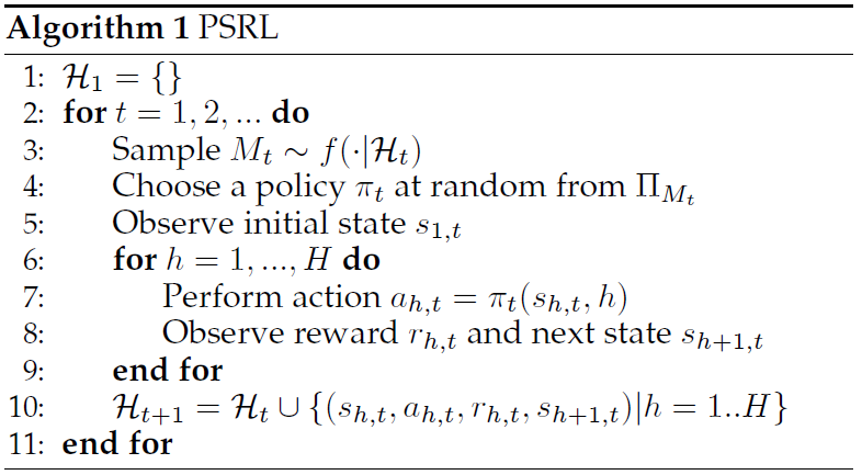
At the beginning of each episode \(t\), a MDP \(M_t\) is sampled from the current posterior. Let \(P_t\) and \(R_t\) be the transition and reward distributions of \(M_t\). The set of optimal policies \(\Pi_{M_t}\) for this MDP can be found using Backward Induction as \(P_t\) and \(R_t\) are known. The agent samples a policy \(\pi_t\) from \(\Pi_{M_t}\) and follows it for \(H\) steps. The rewards and transitions witnessed during this episode are used to update the posteriors. Let \(f\) be the prior density over the MDPs and \(\mathcal{H}_t\) be the history of episodes seen until \(t-1\). Let \(s_{h,t}\) be the state observed, \(a_{h,t}\) be the action performed and \(r_{h,t}\) be the reward received at time \(h\) in episode \(t\).
Similarity to Thompson Sampling
A \(k\)-armed Bernoulli Bandit instance is defined by the unknown \(k\) dimensional vector \((p_1,p_2,..,p_k)\), where \(p_i\) is the probability of success of the \(i\)th arm. Let \(\mathcal{B}_k\) be the set of all \(k\)-armed Bernoulli Bandit. \(\mathcal{B}_k = \{(p_1,p_2,..,p_k):0\leq p_i \leq 1\}\). \(\mathcal{B}_k\) is in fact the \(k\)-dimensional unit cube. Thompson Sampling essentially maintains a probability density over \(\mathcal{B}_k\). At each step, it samples a bandit instance from \(\mathcal{B}_k\) according to this density, acts Optimally with respect to the sampled instance and uses Bayes’s Theorem to update the density according to the rewards received. When the arms are uncorrelated, this procedure corresponds to sampling from each arm separately, i.e., the usual Thompson Sampling algorithm.
Now consider the set of all EFH-MDPs \(\mathcal{M}\) with \(S\) states, \(A\) actions and episode length \(H\). It is a little difficult to visualize the space \(\mathcal{M}\), but it is the product space of a \(SA\) dimensional cube (corresponding to \(R\)) and \(SA\) simplexes of dimension \(S-1\) (corresponding to \(P\)). PSRL maintains a probability density over \(\mathcal{M}\). At each episode, it samples an MDP instance from \(\mathcal{M}\) according to this density, acts Optimally with respect to the sampled instance and uses Bayes’s Theorem to update the density according to the rewards and transitions witnessed.
Posterior Sampling
Posterior Sampling serves as a general idea which transcend both Bandits and MDPs. It can be used for bandits with correlated arms (both known and unknown correlations), contextual bandits and possibly even a general class of problems called Contextual Decision Processes. The idea can be captured in 4 simple lines:
- Maintain a probability density over the space of Models.
- Sample an instance according to this density.
- Act optimally according to the sampled instance.
- Use Bayes’s theorem to update the probability density.
By following these four steps, it is guaranteed that the density will concentrate around the true parameters of the model.
Extra Reading
There is a significant amount of work dedicated to proving that PSRL and similar posterior sampling algorithms are sample efficient and suffer low worst case regret. Section 3.3 of the Bayesian RL book provides a good summary of the current state of these results.