Markov Decision Processes
This blog post is about Episodic Fixed Horizon Markov Decision Processes (EFH-MDP). MDPs are a very generic framework and can be used to model complex systems in manufacturing, control and robotics to state a few. These are also used to model environments in Reinforcement Learning (RL).
There exist several variants of MDPs. This blog post will talk about the Episodic Fixed Horizon version. These can be used when interaction with the MDP lasts for a fixed period of time, as is usually the case in time constrained environments. There is an agent which interacts with the environment and tries to maximize the rewards it receives.
An EFH-MDP \(M\) is given by the tuple \(\langle \mathcal{S},\mathcal{A},R,P,H,\rho \rangle\). Here \(\mathcal{S}=\{ 1,...,S \}\) is a finite set of states and \(\mathcal{A}=\{ 1,...,A \}\) is a finite set of actions. An agent interacts with \(M\) in episodes of length \(H\) steps. In each step \(h=[H] \equiv \{1,2..,H\}\) of an episode, the agent observes a state \(s_h \in \mathcal{S}\) and decides to perform an action \(a_h \in \mathcal{A}\). It then receives a reward \(r_h\) which is sampled from the reward distribution \(R(s_h,a_h)\). If \(h<H\), it also transitions to a new state \(s_{h+1}\) sampled from the transition probability distribution \(P(s_h,a_h)\). If \(h=H\), the episode ends, a state is sampled from the initial state distribution \(\rho\) and a new episode begins.
A policy \(\pi\) is a mapping from \(s \in \mathcal{S}\) and time step \(h=1,...,H\) to action \(a \in A\). A policy basically tells the agent how to behave if it is in state \(s\) at step \(h\) of the episode. The goal of the agent is to find a policy such that its average reward starting from any state \(s\) at any step \(h\) is maximized. Let the policy with the highest average reward be \(\pi^*\). There may exist multiple optimal policies for a given MDP.
\[\pi^* \in \arg\max_{\pi} (\mathbb{E} \big[\sum_{i=h}^H r_i \big| r_i \sim R(s_i,\pi(s_i,i))\big]) \quad \forall (s,h) \in \mathcal{S}\times [H]\]| Let the average reward received for a particular state-action be $$\bar{R}(s,a) = \mathbb{E}[r | r \sim R(s,a)]$$. |
The value of a state \(s\) and action \(a\) under a policy \(\pi\) is defined as the expected sum of rewards attained starting at state \(s\) at step \(h\), performing action \(a\) and acting according to \(\pi\) till the end of the episode.
\[Q_{\pi}(s,a,h) = \mathbb{E}\bigg[\bar{R}(s,a)+\sum_{i=h+1}^{H} \bar{R}(s_i,\pi(s_i,i))\bigg]\]Let \(V_{\pi}(s,h) = Q_{\pi}(s,\pi(s,h),h)\).
\[V_{\pi}(s,h) = \mathbb{E}\bigg[ \sum_{i=h}^{H} \bar{R}(s_i,\pi(s_i,i))\bigg]\]\(Q_{\pi}(s,a,h)\) can be re-written as:
\[\begin{align*} Q_{\pi}(s,a,h) &= \mathbb{E}\bigg[\bar{R}(s,a)+\sum_{i=h+1}^{H} \bar{R}(s_i,\pi(s_i,i))\bigg] \\ &= \bar{R}(s,a)+ \mathbb{E}\bigg[\sum_{i=h+1}^{H} \bar{R}(s_i,\pi(s_i,i))\bigg] \\ &= \bar{R}(s,a) + \sum_{s' \in \mathcal{S}} P(s,a,s')V_{\pi}(s',h+1) \\ &= \bar{R}(s,a) + \sum_{s' \in \mathcal{S}} P(s,a,s')Q_{\pi}(s',\pi(s',h+1),h+1) \end{align*}\]\[Q_{\pi}(s,a,h) = \bar{R}(s,a) + \sum_{s' \in \mathcal{S}} P(s,a,s')V_{\pi}(s',h+1)\]
This is the Bellman Equation.
The optimal policy \(\pi^*\) is given by:
\[\pi^* \in \arg \max_{\pi} V_{\pi}(s,h) \quad \forall (s,h) \in \mathcal{S}\times [H]\]The value of the optimal policy \(V_{\pi^*}(s,h)\) is:
\[V_{\pi^*}(s,h) = Q_{\pi*}(s,\pi^*(s,h),h) = \max_a Q_{\pi^*}(s,a,h)\]\(Q_{\pi^*}(s,a,h)\) can be written as:
\[\begin{align*} Q_{\pi^*}(s,a,h) &= \bar{R}(s,a) + \sum_{s' \in \mathcal{S}} P(s,a,s')V_{\pi^*}(s',h+1) \\ &= \bar{R}(s,a) + \sum_{s' \in \mathcal{S}} P(s,a,s') \max_{a'} Q_{\pi^*}(s',a',h+1) \end{align*}\]\[Q_{\pi^*}(s,a,h) = \bar{R}(s,a) + \sum_{s' \in \mathcal{S}} P(s,a,s') \max_{a'} Q_{\pi^*}(s',a',h+1)\]
This is the Bellman Optimality Equation.
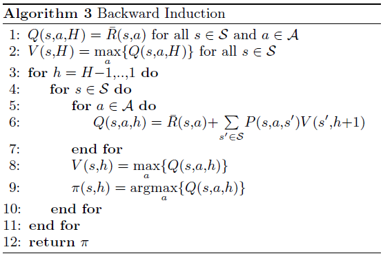
When the rewards and transition probabilities are known, an optimal policy for the MDP can be found using Dynamic Programming. The algorithm iterates backwards from \(h=H\) to \(h=1\), and hence is called as Backward Induction. At \(h=H\), the \(Q\) values for each state-action are equal to their average immediate rewards as it is the end of the episode. At each step, it computes the \(Q\) values by applying the Bellman Operator for each state and action. The time complexity of this algorithm is \(O(S^2AH)\) as applying the Bellman Operator requires \(O(S)\) steps and we do this \(SAH\) times.
A note about Stationarity
In Infinite Horizon Discounted MDPs, the policies are stationary( ie, only dependent on state and not time). In EFH-MDPs, the policies are non stationary as the action depends on the state \(s\) and current step in the episode \(h\). Non stationary policies are necessary for EFH-MDPs. Consider the MDP below. It has 4 states, two actions and horizon length 3 starting from \(s_0\). Choosing to go right from \(s_0\) will end in going to \(s_2\) or remaining in \(s_0\) with equal probability. The only rewards in the system have value \(1\) and \(5\) which are obtained by going left at \(s_1\) and right at \(s_3\) respectively.
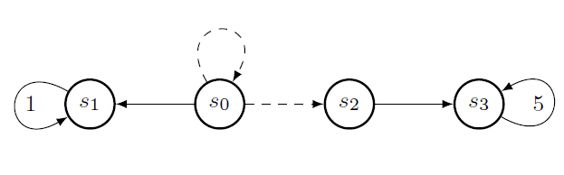
In this MDP, the best stationary policy is to always go right. This policy’s expected total reward per episode is \(2.5\). The best non-stationary policy however is to go right from \(s_0\) at \(h=1\). If it succeeds to go to \(s_2\), then it can get a reward of \(5\) by continuing right until the episode ends. However, if it remain in \(s_0\), it can get a reward of \(1\) by going left until the episode ends. Hence the expected total reward for the best non-stationary policy is \(3\).