From Potentials to Probabilities
This post is about “Potential Functions” in the context of Online Learning. These form the basis for the Implicitly Normalized Forecaster(INF) studied in [1,2]. We present some basic results about potential functions here.
A function \(\psi: (-\infty,a) \to (0,+\infty)\) for some \(a \in \mathbb{R} \cup \{+\infty\}\) is called a potential if it is convex, continuously differentiable and satisfies:
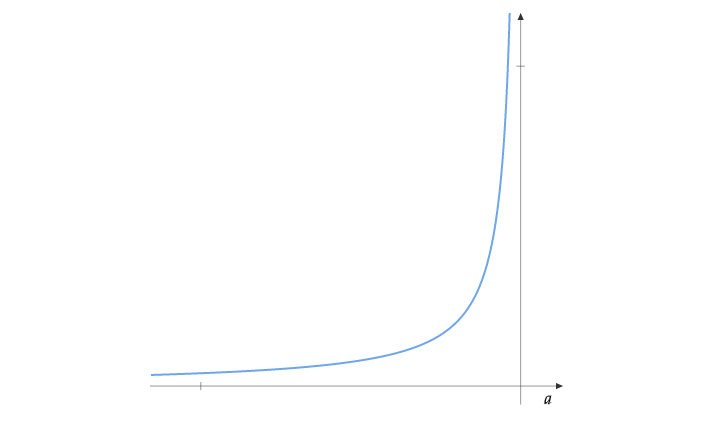
\[\begin{align*} \lim_{x \to -\infty} \psi(x) = 0 \quad &&\quad \lim_{x \to a} \psi(x) = +\infty\\ \psi' >0 \quad && \quad \int_{0}^{1} |\psi^{-1} (s)| ds < + \infty \end{align*}\]For instance, \(\exp(x)\) is a potential function with \(a=\infty\) and \(-1/x\) is a potential with \(a=0\). A potential function usually looks like this:
Consider a function \(g: \mathbb{R}^n \times \mathbb{R} \to \mathbb{R}_+\) defined as
\[g(y,\lambda) = \sum_{i=1}^n \psi(y_i + \lambda)\]Lemma 1: For every \(y \in \mathbb{R}^n\), there exists a unique \(\lambda\) such that \(y_i + \lambda < a\) for all \(i\) and \(g(y, \lambda)=1\)
Proof: For every \(y \in \mathbb{R}^n\), we have that \(\lim_{\lambda \to -\infty} g(y,\lambda) = 0\) and \(\lim_{\lambda \to a-\min_i(y_i)} g(y,\lambda) = +\infty\). As \(g\) is monotonically increasing and continuous, by the intermediate value theorem, for every \(y \in \mathbb{R}^n\) there exists a unique \(\lambda\) such that \(g(y, \lambda)=1\).
Using Lemma 1, we can define a function \(\lambda(y)\) such that:
\[g(y,\lambda(y)) = \sum_{i=1}^n \psi(y_i + \lambda(y))=1\]Q.E.D
Since \(\psi(y_i + \lambda(y)) \geq 0\) and \(\sum_{i=1}^n \psi(y_i + \lambda(y))=1\), we can see that \(P(y) = \{\psi(y_i + \lambda(y))\}_{i=1}^n\) forms a probability distribution.
These probability distributions defined through \(\psi\) come up in online learning algorithms such as OMD and FTRL when the decision space is the probability simplex. A generalized Implicitly Normalized Forecaster(INF) algorithm can be written as:
Generalized INF Given a potential \(\psi\) and “Loss Aggregators” \(h_1,h_2,\dots,h_T\)
- Let \(\theta_0 = 0\)
- For \(t=1 \dots T:\)
- Play the point \(x_t = P(\theta_{t-1}) = \psi(\theta_{t-1} + \lambda(\theta_{t-1}))\)
- Observe the loss function \(l_t(x)\)
- Compute \(\theta_t = h_t(l_1,\dots,l_t)\)
The loss aggregators collect the losses seen so far and output a vector, using which we compute the point to play.
Considering linear losses, the aggregators for time varying OMD are given by:
\[h_t(l_1,\dots,l_t) = - \sum_{s=1}^t \eta_s l_s\]The aggregators for time varying FTRL are given by:
\[h_t(l_1,\dots,l_t) = - \eta_t \sum_{s=1}^t l_s\]We will treat OMD and FTRL in future posts. In the remaining post, we present some properties of potential functions.
Constant Translation
Lemma 2: Let \(y, y' \in \mathbb{R}^n\). If \(y'_i = y_i + c\) for all \(i\), then \(\lambda(y') = \lambda(y)-c\).
Proof: Observe that
\[g(y, c+\lambda(y')) =\sum_{i=1}^n \psi(y_i +c + \lambda(y')) = \sum_{i=1}^n \psi(y'_i + \lambda(y')) = g(y',\lambda(y'))= 1\]Since \(\lambda(y)\) is the unique solution to \(g(y,\lambda)=1\), we must have that \(\lambda(y) = c + \lambda(y')\).
Q.E.D
Associated Function
Associated with a potential \(\psi\), we define a function \(f:(0,+\infty) \to \mathbb{R}\) as
\[f(z) = \int_{0}^z \psi^{-1}(s) ds\]Observe that \(f'(z) = \psi^{-1}(z)\) and \(f'(z) = \left[ \psi'(\psi^{-1}(z))\right]^{-1}\). So \(\lim_{z \to 0}\mid \psi^{-1}(z)\mid = +\infty\) and \(f\) is strictly convex, proving that \(f\) is a Legendre function on \((0,\infty)\). The Legendre-Fenchel dual of \(f\) is \(f^\star:(-\infty,a) \to \mathbb{R}\) defined as \(f^\star(u) = \sup_{z > 0} zu - f(z)\), which by definition of \(f\) is same as:
\[f^\star(u) = u \psi(u) - f(\psi(u))\]The following relations hold:
\[\begin{align*} f'(z) = \psi^{-1}(z) \quad && \quad {f^\star}'(u) = \psi(u) \\ f''(z) = \left[ \psi'(\psi^{-1}(z))\right]^{-1} \quad && \quad {f^\star}''(u) = \psi'(u) \end{align*}\]The INF algorithm using potential \(\psi\) along with suitable aggregators will be equivalent to OMD/FTRL on the simplex with regularizer \(F(x) = \sum_{i=1}^n f(x_i)\).
Concavity of \(\lambda(y)\)
Taking the gradient of \(\sum_{i=1}^n \psi(y_i + \lambda(y))=1\), we have:
\[\begin{align*} &\sum_{i=1}^n \psi'(y_i+\lambda(y))(e_i + \nabla \lambda(y))=0\\ \implies & \nabla \lambda(y) = - \frac{ \sum_{i=1}^n \psi'(y_i+\lambda(y)) e_i}{\sum_{i=1}^n \psi'(y_i+\lambda(y))} \end{align*}\]\(\nabla \lambda(y)\) is the vector \(\{- \frac{ \psi'(y_i+\lambda(y)) }{\sum_{i=1}^n \psi'(y_i+\lambda(y))}\}_{i=1}^n\).
Taking the gradient of \(\sum_{i=1}^n \psi'(y_i+\lambda(y))(e_i + \nabla \lambda(y))=0\), we have:
\[\begin{align*} &\sum_{i=1}^n \psi''(y_i+\lambda(y))(e_i + \nabla \lambda(y))^{\otimes 2} + \nabla^2 \lambda(y) \left(\sum_{i=1}^n \psi'(y_i+\lambda(y)) \right)=0\\ \implies & \nabla^2 \lambda(y) = - \frac{ \sum_{i=1}^n \psi''(y_i+\lambda(y))(e_i + \nabla \lambda(y))^{\otimes 2} }{\sum_{i=1}^n \psi'(y_i+\lambda(y))} \end{align*}\]The above Hessian is negative definite, so \(\lambda(y)\) is strictly concave.
Convexity of \(D(y)\)
Define the function:
\[D(y) = -\lambda(y) + \sum_{i=1}^n f^\star(y_i + \lambda(y))\]The gradient of \(D\) is:
\[\begin{align*} \nabla D(y) &= - \nabla \lambda(y) + \sum_{i=1}^n \psi(y_i + \lambda(y))(e_i + \nabla \lambda(y))\\ &= - \nabla \lambda(y) +\nabla \lambda(y) + \sum_{i=1}^n \psi(y_i + \lambda(y))e_i\\ &= P(y) \end{align*}\]The Hessian of \(D\) is:
\[\begin{align*} \nabla^2 D(y) &= - \nabla^2 \lambda(y) + \sum_{i=1}^n \psi'(y_i + \lambda(y))(e_i + \nabla \lambda(y))^{\otimes 2} + \sum_{i=1}^n \psi(y_i+\lambda(y)) \nabla^2 \lambda(y)\\ &= \sum_{i=1}^n \psi'(y_i + \lambda(y))(e_i + \nabla \lambda(y))^{\otimes 2} \end{align*}\]So \(D(y)\) is strictly convex.
Refernces
[1] Audibert, J. Y., Bubeck, S., & Lugosi, G. (2011, December). Minimax policies for combinatorial prediction games. In Proceedings of the 24th Annual Conference on Learning Theory (pp. 107-132). JMLR Workshop and Conference Proceedings.
[2] Audibert, J. Y., Bubeck, S., & Lugosi, G. (2014). Regret in online combinatorial optimization. Mathematics of Operations Research, 39(1), 31-45.
Parts of this post appear in my paper : Putta, S. R., & Agrawal, S. (2021). Scale Free Adversarial Multi Armed Bandits. arXiv preprint arXiv:2106.04700.