Online Portfolio Selection - Exponentiated Gradient
I presented Cover’s universal portfolio algorithm in my last blog. It has a regret bound of \(O(n \log T)\), where \(n\) is the number of stocks and \(T\) is the number of days traded. I implemented it for the case of two stocks. In the case of large \(n\), Cover’s algorithm can be run using a Markov Chain Monte Carlo simulation. The computation time for this scales as \(O(n^4 T^{14})\), which is quite prohibitive for even moderate \(n\) and \(T\). So, in this blog, I present a gradient descent-based algorithm that trades off computation time with regret bound while still staying universal.
Simple Regret Bound
Define \(f_t(x) = -\log(r_t^\top x)\). Then the regret of a strategy \(Alg\) against a fixed portfolio vector \(x\) is:
\[\mathcal{R}_T(Alg,[r]_1^T,x) = \sum_{t=1}^T \log(r_t^\top x) - \log(r_t^\top x_t) = \sum_{t=1}^T f_t(x_t)-f_t(x)\]Since \(f_t\) is convex in \(x\), we have the simple upper bound:
\[f_t(x_t)-f_t(x) \leq \nabla f_t(x_t)^\top (x_t-x)\]So, we have the regret bound:
\[\sum_{t=1}^T f_t(x_t)-f_t(x) \leq \sum_{t=1}^T \nabla f_t(x_t)^\top (x_t-x)\]The above process is called “linearizing,” as we are linearizing the loss function
\[f_t(x) \approx f_t(x_t) + \nabla f_t(x_t)^\top (x-x_t)\]Linearized Follow-The-Regularized-Leader
We could use a strategy that just uses gradients \(\nabla f_t(x_t) = -\frac{r_t}{r_t^\top x_t}\) instead of the function \(f_t(x)\) for its update.
In my first blog, I mention the Follow-The-Leader (FTL) algorithm. After seeing the returns \(r_1,\dots,r_{t-1}\), it picks the current portfolio vector \(x_t\) as:
\[x_t = \arg\max_{x \in \Delta_n} \sum_{i=1}^{t-1} \log(x^\top r_i) = \arg \min_{x \in \Delta_n} \sum_{i=1}^{t-1} f_i(x)\]The linearized version of FTL is:
\[x_t = \arg \min_{x \in \Delta_n} \sum_{i=1}^{t-1} \nabla f_i(x_i)^\top x\]Since this is a linear function in \(x\), it is minimized at one of the vertices of \(\Delta_n\). It is a well-known fact that FTL on linear losses could incur \(O(T)\) regret (See Example 2.10 in A Modern Introduction to Online Learning). This is because FTL could jump from one vertex to another at every iteration, making it unstable.
One way to stabilize linearized FTL is by adding convex regularization. This algorithm is called linearized Follow-The-Regularized-Leader (FTRL).
\[x_t = \arg \min_{x \in \Delta_n}\left[ R(x) + \eta_t \sum_{i=1}^{t-1} \nabla f_i(x_i)^\top x \right]\]Here \(R(x)\) is the convex regularizer, and \(\eta_t\) is the learning rate.
Exponentiated Gradient Descent
Picking the right regularizer for a problem is an art. Choosing a regularizer that conforms to the geometry of the problem is a good starting point. In this case, since the domain is \(\Delta_n\), a suitable regularizer is negative Shannon entropy.
\[R(x) = \sum_{j=1}^n x[j] \log(x[j])\]This choice gives rise to a closed-form expression for \(x_t\):
\[x_t[j] = \frac{\exp(-\eta_t\sum_{i=1}^{t-1} \nabla f_i(x_i)[j])}{\sum_{k=1}^n \exp(-\eta_t\sum_{i=1}^{t-1} \nabla f_i(x_i)[k])} = \frac{\exp(\eta_t\sum_{i=1}^{t-1} \frac{r_i[j]}{r_i^\top x_i})}{\sum_{k=1}^n \exp(\eta_t\sum_{i=1}^{t-1} \frac{r_i[k]}{r_i^\top x_i})}\]If we choose a constant learning rate \(\eta_t = \eta\), it further simplifies to:
\[x_t[j] =\frac{x_{t-1}[j]\exp(-\eta \nabla f_{t-1}(x_{t-1})[j])}{\sum_{k=1}^n x_{t-1}[k]\exp(-\eta \nabla f_{t-1}(x_{t-1})[k])}= \frac{x_{t-1}[j]\exp(\eta \frac{r_{t-1}[j]}{r_{t-1}^\top x_{t-1}})}{\sum_{k=1}^n x_{t-1}[k]\exp(\eta \frac{r_{t-1}[k]}{r_{t-1}^\top x_{t-1}})}\]This is the Exponentiated Gradient (EG) method, which is the subject of the paper On-Line Portfolio Selection Using Multiplicative Updates.
Regret Bound
If the returns are uniformly lowerbounded by a known constant \(r\), i.e., if for all \(i \in [n]\) and \(t \in [T]\):
\[1\geq r_t[i]\geq r>0\]Then picking \(\eta = 2r \sqrt{2 \log(n)/T}\) in EG, we get the regret bound:
\[\mathcal{R}_T(EG(\eta),[r]_1^T,x) \leq \sum_{t=1}^{T} \nabla f_t(x_t)^\top (x_t-x) \leq \frac{1}{r} \sqrt{\frac{1}{2}T\log(n)}\]For this choice of \(\eta\), we need to know \(T\) and \(r\) beforehand.
If \(T\) is unknown, we can use the changing learning rate \(\eta_t = r\sqrt{\log(n)/t}\) in EG. We get the same regret bound with different leading constants.
\[\mathcal{R}_T(EG(\eta_t),[r]_1^T,x) \leq O\left(\frac{1}{r} \sqrt{T\log(n)}\right)\]Further, if \(r\) is also unknown, we can employ an adaptive algorithm called AdaHedge. We get an adaptive regret bound:
\[\mathcal{R}_T(AdaHedge,[r]_1^T,x) \leq O\left(\sqrt{\log(n)\left(\sum_{t=1}^T \frac{1}{(\min_i r_t[i])^2}\right)}\right)\]For further details about AdaHedge, see section 7.5 and section 7.6 in A Modern Introduction to Online Learning.
We need to modify the EG algorithm to completely remove the dependence on \(r\) in the regret bound. Instead of using the actual returns \(r_{1},\dots,r_T\) to update the algorithm, we use the perturbed returns:
\[\tilde{r}_t = \left(1- \frac{\alpha_t}{n}\right)r_t + \frac{\alpha_t}{n} \textbf{1}\]The \(EG(\eta_t)\) update is:
\[x_t[j] = \frac{\exp(\eta_t\sum_{i=1}^{t-1} \frac{\tilde{r}_i[j]}{\tilde{r}_i^\top x_i})}{\sum_{k=1}^n \exp(\eta_t\sum_{i=1}^{t-1} \frac{\tilde{r}_i[k]}{\tilde{r}_i^\top x_i})}\]Instead of picking the portfolio \(x_t\), we select the perturbed portfolio:
\[\tilde{x}_t[j] = (1-\alpha_t) x_t[j] + \frac{\alpha_t}{n}\]The resultant algorithm is \(\widetilde{EG}\). With the choice \(\eta_t = \frac{\alpha_t}{n} \sqrt{\frac{\log(n)}{t}}\) and \(\alpha_t = n^{1/2} (\log n)^{1/4} t^{-1/4}\), it is possible to show that:
\[\mathcal{R}_T(\widetilde{EG}(\eta_t,\alpha_t),[r]_1^T,x) \leq O\left(n^{1/2} (\log n)^{1/4} T^{3/4}\right)\]Since this bound holds for any \(T\) and sequence of returns, \(\widetilde{EG}(\eta_t,\alpha_t)\) is a universal portfolio algorithm. Its regret is much larger than Cover’s universal portfolio, whose regret is \(O(n\log T)\). However, its iteration runtime is \(O(n)\), which is much better compared to Cover’s runtime of \(O(n^4 T^{14})\). A variant of \(\widetilde{EG}(\eta_t,\alpha_t)\) appears in On-Line Portfolio Selection Using Multiplicative Updates.
Experiments
In the code below, I implement linearized FTL, AdaHedge, and \(\widetilde{EG}\)
References
- The EG algorithm was introduced in the paper On-Line Portfolio Selection Using Multiplicative Updates.
- The AdaHedge algorithm is by De Rooij, Steven et al. “Follow the leader if you can, hedge if you must.” The Journal of Machine Learning Research 15.1 (2014): 1281-1316. A simplified analysis for AdaHedge can be found in A Modern Introduction to Online Learning as well as the blog AdaHedge.