Online Mirror Descent
In this blog post, we introduce OMD and state an upperbound for its regret. Using this upperbound, we analyze the regret of the algorithm we proposed in our previous blog.
OMD can also be thought of as a game between a player and an adversary which proceeds as follows:
- For \(t=1...T\)
- Player chooses a point \(x_t\) from a convex set \(\mathcal{K}\)
- The adversary simultaneously reveals a convex function \(f_t\) to the player.
- The player suffers the loss \(f_t(x_t)\)
Like before, the goal of the player is to minimize the regret:
\[\sum_{t=1}^T f_t(x_t) - \min_{x^\star \in \mathcal{K}}\sum_{t=1}^T f_t(x^\star)\]To understand OMD, we need to introduce Bregman Divergences and Fenchel Conjugates.
Bregman Divergence
Let \(R(x)\) be a convex function. The Bregman Divergence \(D_R(x\|y)\) is:
\[D_R(x\|y) = R(x)-R(y)-\langle \nabla R(y),x-y\rangle\]In words, \(D_R(x\|y)\) is the difference between \(R(x)\) and the first order approximation of \(R(x)\) from \(y\), which is \(R(y)+\langle \nabla R(y),x-y\rangle\). As a consequence of convexity, \(D_R(x\|y) \geq 0\).
Fenchel Conjugate
The Fenchel Conjugate of \(R(x)\) is defined as:
\[R^\star(\theta) = \max_x \langle x,\theta \rangle - R(x)\]From its definition, we have \(R^\star(\theta) +R(x) \geq \langle x,\theta \rangle\), which is the Fenchel-Young inequality.
Online Mirror Descent
The OMD algorithm uses a convex regularization function \(R(x)\). The algorithm is as follows:
- The player picks \(y_1\) such that \(\nabla R(y_1)=0\) and \(x_1 = \arg \min \limits_{x\in \mathcal{K}} D_R(x\|y_1)\)
- For \(t=1...T\)
- Player chooses the point \(x_t\)
- The player sees \(f_t\) and suffers the loss \(f_t(x_t)\)
- Update \(y_{t+1}\) \(\nabla R(y_{t+1}) = \nabla R(x_{t}) - \eta \nabla f_t(x_t)\)
- Project back to \(\mathcal{K}\) \(x_{t+1} = \arg \min \limits_{x\in \mathcal{K}} D_R(x\|y_{t+1})\)
We state the regret inequality for OMD, as derived in Regret Analysis of Stochastic and Nonstochastic Multi-Armed Bandit Problems
\[\sum_{t=1}^T f_t(x_t) - \sum_{t=1}^T f_t(x) \leq \frac{R(x) - R(x_1)}{\eta} + \frac{1}{\eta} \sum_{t=1}^T D_{R^\star}(\nabla R(x_{t}) - \eta \nabla f_t(x_t)\| \nabla R(x_{t}))\]Online Combinatorial Optimization
We apply OMD to the OCO problem from the previous blog post. Here \(f_t(x) = \langle l_t,x\rangle\), so \(\nabla f_t(x) = l_t\). We use the following regularizer:
\[R(x) = \sum_{i=1}^n x_i\log x_i +(1-x_i) \log (1-x_i)\]Its gradient is:
\[\nabla R(x)_i = \log \frac{x_i}{1-x_i}\]Hence, we have the following update:
\[\begin{align} \log \frac{y_{t+1,i}}{1-y_{t+1,i}} &= \log \frac{x_{t,i}}{1-x_{t,i}} - \eta l_{t,i}\\ \frac{y_{t+1,i}}{1-y_{t+1,i}} &= \frac{x_{t,i}}{1-x_{t,i}} \exp(-\eta l_{t,i})) \\ y_{t+1,i} &= \frac{x_{t,i}}{x_{t,i} + (1-x_{t,i})\exp(\eta l_{t,i})} \end{align}\]Since \(y_{t,i}\) is always in \([0,1]\), we can skip the Bregman projection step. Hence, we have:
\[x_{t+1,i} = \frac{x_{t,i}}{x_{t,i} + (1-x_{t,i})\exp(\eta l_{t,i})} = \frac{1}{1+\exp(\eta \sum_{\tau=1}^tl_{\tau,i})}\]This is the same update we had used in our algorithm to do Hedge in linear time. Now we analyze the expected regret of our algorithm using OMD’s regret:
\[\begin{align} \mathbb{E}[R_T] &= \mathbb{E}[\sum_{t=1}^TL_t(X_t)] - \min_{X^\star \in \{0,1\}^n} \sum_{t=1}^TL_t(X^\star)\\ &=\mathbb{E}[\sum_{t=1}^T \langle l_t,X_t\rangle] - \min_{X^\star \in \{0,1\}^n}\sum_{t=1}^T \langle l_t,X^\star\rangle \end{align}\]Recall that \(\Pr(X_t=X) = \prod_{i=1}^n (x_{t,i})^{X_i}(1-x_{t,i})^{1-X_i}\). Hence, we have \(\mathbb{E}[\sum_{t=1}^T \langle l_t,X_t\rangle] = \sum_{t=1}^T \langle l_t,x_t\rangle\). Using OMD’s regret inequality, we get:
\[\begin{align} \mathbb{E}[R_T]&= \sum_{t=1}^T \langle l_t,x_t\rangle - \min_{X^\star \in \{0,1\}^n}\sum_{t=1}^T \langle l_t,X^\star\rangle\\ &\leq \frac{R(X^\star) - R(x_1)}{\eta} + \frac{1}{\eta} \sum_{t=1}^T D_{R^\star}(\nabla R(x_{t}) - \eta l_t\| \nabla R(x_{t})) \end{align}\]The first term can be bounded very easily \(R(X^\star) - R(x_1) \leq n \log 2\). The second term is a little involved:
\[\begin{align} D_{R^\star}(\nabla R(x_{t}) - \eta l_t\| \nabla R(x_{t})) &= D_{R^\star}(-\eta \sum_{\tau=1}^tl_\tau\| -\eta \sum_{\tau=1}^{t-1}l_\tau)\\ &=R^\star(-\eta \sum_{\tau=1}^tl_\tau) - R^\star(-\eta \sum_{\tau=1}^{t-1}l_\tau) + \langle \nabla R^\star(-\eta \sum_{\tau=1}^{t-1}l_\tau),\eta l_t\rangle \end{align}\]The Fenchel Conjugate of \(R(x)\) is:
\[R^\star(\theta) = \max_{x \in [0,1]^n} \langle x,\theta \rangle - R(x)\]Differentiating \(\langle x,\theta \rangle - R(x)\) wrt \(x_i\) and equating to \(0\),
\[\begin{align} \theta_i - \log x_i + \log(1-x_i) &= 0\\ \frac{x_i}{1-x_i} &=\exp(\theta_i) \\ x_i &= \frac{\exp(\theta_i)}{1+\exp(\theta_i)} \end{align}\]Substituting this back in the expression for \(R^\star(\theta)\), we get:
\[R^\star(\theta) = \sum_{i=1}^n \log (1+\exp(\theta))\]Its gradient is:
\[\nabla R^\star(\theta)_i = \frac{\exp(\theta_i)}{1+\exp(\theta_i)}\]We can simplify \(\langle \nabla R^\star(-\eta \sum_{\tau=1}^{t-1}l_\tau),\eta l_t\rangle\) by observing that:
\[\nabla R^\star(-\eta\sum_{\tau=1}^{t-1}l_\tau)_i = \frac{1}{1+\exp(\eta \sum_{\tau=1}^{t-1}l_{\tau,i})} = x_{t,i}\]Simplifying the Bregman term:
\[\begin{align} D_{R^\star}(\nabla R(x_{t}) - \eta l_t\| \nabla R(x_{t})) &=\bigg(\sum_{i=1}^n \log \frac{1+\exp(-\eta \sum_{\tau=1}^{t}l_{\tau,i})}{1+\exp(-\eta \sum_{\tau=1}^{t-1}l_{\tau,i})} \bigg)+ \eta\langle x_t,l_t\rangle\\ &=\bigg(\sum_{i=1}^n \log \frac{1+\exp(\eta \sum_{\tau=1}^{t}l_{\tau,i})}{\exp(\eta l_{t,i})(1+\exp(\eta \sum_{\tau=1}^{t-1}l_{\tau,i}))}\bigg)+ \eta\langle x_t,l_t\rangle \end{align}\]Using the fact that \(x_{t,i} = (1+\exp(\eta \sum_{\tau=1}^{t-1}l_{\tau,i}))^{-1}\),
\[\begin{align} &=\bigg(\sum_{i=1}^n \log \frac{x_{t,i}+(1-x_{t,i})\exp(\eta l_{t,i})}{\exp(\eta l_{t,i})}\bigg)+ \eta\langle x_t,l_t\rangle\\ &=\sum_{i=1}^n \log(1-x_{t,i}+x_{t,i}\exp(-\eta l_{t,i})) + \eta\langle x_t,l_t\rangle \end{align}\]Using the inequality: \(e^{-a} \leq 1-a+a^2\)
\[\leq \sum_{i=1}^n \log(1-\eta x_{t,i}l_{t,i}+\eta^2 x_{t,i}l_{t,i}^2) + \eta\langle x_t,l_t\rangle\]Using the inequality: \(\log(1-a) \leq -a\)
\[\leq -\eta \langle x_t,l_t\rangle+\eta^2 \langle x_t,l_t^2\rangle +\eta \langle x_t,l_t\rangle = \eta^2 \langle x_t,l_t^2\rangle\]The second term is \(\eta\sum_{t=1}^T\langle x_t,l_t^2\rangle\). So the regret inequality is:
\[\mathbb{E}[R_T] \leq \frac{n \log 2}{\eta} + \eta\sum_{t=1}^T\langle x_t,l_t^2\rangle\]Since \(l_{t,i} \in [-1,+1]\) and \(x_t \in [0,1]^n\), we get \(\mathbb{E}[R_T]\leq \frac{n \log 2}{\eta} + \eta Tn\). Substituting \(\eta = \sqrt{\frac{log 2}{T}}\), we get \(\mathbb{E}[R_T]\leq 2n\sqrt{T \log2}\).
In the previous blog post, we showed that Hedge and our algorithm are equivalent. In this post, we showed that OMD with Entripic regularization and our algorithm are equivalent. Hence, in this particular case, Hedge, OMD+Entripic regularization and our algorithm are the same and have expected regret bounded by \(O(n\sqrt{T})\). This is because our decision space was all \(2^n\) points in \(\{0,1\}^n\) and so, we were able to factorize Hedge’s update and sampling steps. In general, this is not always possible. For instance, if our decision space was \(\mathcal{S}_m = \{X: \|X\|_1 \leq m, X \in \{0,1\}^n \}\). We would not have been able to factorize Hedge’s update like we did in our algorithm.