Multi Armed Bandits and Exploration Strategies
This blog post is about the Multi Armed Bandit(MAB) problem and about the Exploration-Exploitation dilemma faced in reinforcement learning. MABs find applications in areas such as advertising, drug trials, website optimization, packet routing and resource allocation.
A Multi Armed Bandit consists of \(K\) arms, \(K\ge2\) numbered from \(1\) to \(K\). Each arm \(a\) is associated with an unknown probability distribution \(P_a\) whose mean is \(\mu_a\). Pulling the \(a\)th arm produces a reward \(r\) which is sampled from \(P_a\). There is an agent which has a budget of \(T\) arm pulls. The agent has to pull these arms in some sequence so as to maximize the accumulated reward after \(T\) arm pulls. The reward for pulling arm \(a_i\) at the \(t\)‘th step be \(r_{a_i,t}\) which is sampled from \(P_{a_i}\). The agent’s task is to maximise \(\sum_{t=1}^T r_{a_i,t}\).
\[Maximize \quad \sum_{t=1}^T r_{a_i,t} \quad \mbox{where } r_{a_i,t} \sim P_{a_i}\]Since the arm rewards are stochastic, we concentrate on maximising the expected total reward.
\[\mbox{Total Reward}= \sum_{t=1}^T r_{a_i,t}\] \[\begin{align*} E[\mbox{Total Reward}] &= E\big[\sum_{t=1}^T r_{a_i,t}\big]\\ &=\sum_{t=1}^T E[r_{a_i,t}]\\ &=\sum_{t=1}^T\mu_{x_t} \end{align*}\]Where \(x_t \in \{a_1,a_2,..,a_K\}\) for \(t=1,2,..T\) are the sequence of arm pulls.
The arm which has the highest mean reward is called as the optimal arm. Let \(a^*\) be the optimal arm and \(\mu^*\) be its mean reward. Another way of maximizing the cumulative reward is by minimizing the cumulative expected Regret.
\[Regret = \sum_{t=1}^Tr_{a^*,t}-r_{a_i,t}\] \[\begin{align*} E[Regret]&=E\big[\sum_{t=1}^Tr_{a^*,t}-r_{a_i,t}\big]\\ &=\sum_{t=1}^TE[r_{a^*,t}] - \sum_{t=1}^TE[r_{a_i,t}] \\ &= T\mu^* - \sum_{t=1}^T\mu_{x_t} \end{align*}\]So the agent can minimize the cumulative expected regret if it can identify the optimal arm. Initially the agent does not know anything about the distribution of the rewards of each arm. It has to explore by pulling the arms in some sequence and has to learn these distributions. Also the agent has to exploit by pulling the arm which it believes to be the most rewarding, as its goal is to maximize the cumulative reward. But how does the agent decide when to explore and when to exploit? This is the exploration-exploitation dilemma. Explore too much and the agent will accumulate less reward. Exploit too much and the agent may not discover the optimal arm and still accumulate less reward.
Let \(Q_a\) represent the empirical mean of the rewards received by pulling arm \(a\). \(Q_a\) is an unbiased estimate of \(\mu_a\)
\[Q_a = \frac{\mbox{Sum of rewards received from arm }a}{\mbox{Number of times arm }a \mbox{ was pulled} }\]The kind of MAB we consider here is the Stochastic multi armed bandit. In this case, the support of the probability distribution \(P_a\) is \([0,1]\), so naturally \(\mu_a\) and the rewards for each arm are bounded between \([0,1]\). A sub case of Stochastic bandits are Bernoulli bandits, in which the rewards are either \(0\) or \(1\) and the probability distribution \(P_a\) is a Bernoulli distribution with unknown success probability \(\mu_a\).
The algorithm for Bernoulli MAB is as follows:
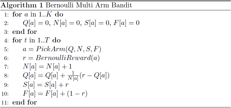
Here \(Q[a]\) is the empirical average reward of pulling arm \(a\), \(N[a]\) is the number of times arm \(a\) was pulled, \(S[a]\) is the number of times a reward of \(1\) was received when arm \(a\) was pulled and \(F[a]\) is the number of times a reward of \(0\) was received when arm \(a\) was pulled.
Now we have to decide how to pick an arm so as to balance exploration and exploitation so that the cumulative reward is maximized.
Random Selection
Pick the arm completely at random. This is not an effective strategy as it completely disregards the history of the arm pulls. We only consider pulling random arms to form a baseline to compare it with other strategies. The expected cumulative regret for random arm selection would be:
\[E[Regret] = T\mu^* - \sum_{t=1}^TE[r_{a_i,t}] = T(\mu^* - \bar{\mu})\]Here \(\bar{\mu}\) is the mean of \(\mu_1,\mu_2,..,\mu_K\). The regret is linear in the number of arm pulls.
Greedy Selection
Pick the arm which has the highest empirical average reward breaking ties randomly.
\[A = argmax_a (Q[a])\]Note that initially, all \(Q[a]\) are \(0\), so arms are selected randomly until one of the arms give a non zero reward. Form then on only that arm will be chosen. This strategy does no exploration at all and so it is very unlikely that the optimal arm is selected. The expected cumulative regret for greedy arm selection would be:
\[E[Regret] = T\mu^* - \sum_{t=1}^TE[r_{a_i,t}] = T(\mu^* - \mu_{a_{i'}})\]Here \(a_{i'}\) is the first arm which produces a non zero reward. Since any of the \(K\) arms could be the first to give a non zero reward, we take the expectation over them. This gives the same linear regret as random selection.
\(\epsilon\)-Greedy Selection
With some probability \(\epsilon\), \(0<\epsilon<1\), pick a random arm. Otherwise with probability \(1-\epsilon\) pick the greedy arm. So the probability of picking the greedy arm would be \(1-\epsilon +\frac{\epsilon}{K}\) and any other arm is picked with probability \(\frac{\epsilon}{K}\)
\[P(a_i)=\begin{cases} 1-\epsilon +\frac{\epsilon}{K} & \mbox{, if } a_i = argmax_a (Q[a])\\ \frac{\epsilon}{K} &\mbox{, otherwise} \end{cases}\]Consider the case where \(\epsilon\) is constant. The expected cumulative regret would be:
\[\begin{align*} E[Regret] &= \sum_{t=1}^TE[r_{a^*,t}] - \sum_{t=1}^TE[r_{a_i,t}] \\ &\ge\sum_{t=1}^T \mu^*-[(1-\epsilon)\mu^* +\epsilon\bar{\mu}]\\ &= T\epsilon(\mu^* - \bar{\mu}) \end{align*}\]The regret is again linear in the number of arm pulls.
We could change \(\epsilon\) through time so that the agent acts greedily in the limit as \(T\to \infty\). Initially the agent should behave randomly to encourage exploration and, as time progresses, it should act more greedily. It is possible to achieve logarithmic regret using a decaying \(\epsilon\)-greedy strategy, but decay schedule requires the knowledge of \(P_i\)s.
Boltzmann Exploration
A problem with the \(\epsilon\)-greedy strategy is that it treats all of the arms, apart from the best arm, equivalently. We could select arm \(a\) with a probability depending on the value of \(Q[a]\). This is known as a soft-max action selection. A common method is to use a Boltzmann distribution, where the probability of selecting arm \(a\) is proportional to \(\exp(Q[a]/\tau)\). That is, the agent selects arm \(a\) with probability
\[P(a) = \frac{\exp(Q[a]/\tau)}{\sum_a \exp(Q[a]/\tau)}\]where \(\tau>0\) is the temperature specifying how randomly arms should be chosen. When \(\tau\) is high, the arms are chosen in almost equal amounts. As the temperature is reduced, the highest-valued arms are more likely to be chosen and, in the limit as \(\tau\to0\), the best arm is always chosen. The expected cumulative regret for Boltzmann Exploration is also linear.
Upper-Confidence-Bound Arm Selection
This strategy is based on the Optimism in the Face of Uncertainty principle. We know that \(Q[a]\) is an unbiased estimate of \(\mu_a\). After some \(N[a]\) pulls of arm \(a\) we can be fairly certain about how close \(Q[a]\) is to \(\mu_a\). Using Hoeffding’s Inequality which we used in my previous post we can derive the following bound:
\[\Pr(\mid Q[a] - \mu_a \mid \ge \epsilon)\le 2 \exp(-2N[a]\epsilon^2)\]Using a one sided version of this inequality we get:
\[\Pr(\mu_a \ge Q[a] + \epsilon) \le \exp(-2N[a]\epsilon^2)\]So for arm \(a\), whose average reward is \(Q[a]\) after it has been pulled \(N[a]\) times, \(\mu_a\) exceeds the upper confidence bound(UCB) with probability \(p = \exp(-2N[a]\epsilon^2)\)
We want the probability that \(\mu_a\) exceeds UCB to decrease with \(t\), the number of arm pulls so far. We could use \(p=t^{-4}\), which ensures that we select the optimal action in the limit as \(t \to \infty\).
\[\epsilon = \sqrt{\frac{-\log p}{2N[a]}} = \sqrt{\frac{2\log t}{N[a]}}\]The UCB strategy is as follows:
\[A = argmax_a\bigg[ Q[a] +\sqrt{\frac{2\log t}{N[a]}} \bigg]\]The UCB strategy could also be seen as an Incentive Based exploration strategy. Here the extra incentive apart from the expected reward for pulling arm \(a\) is \(\sqrt{\frac{2\log t}{N[a]}}\) which could be interpreted as the reward for gaining confidence about arm \(a\)’s reward. This incentive may cause the agent to pull non-greedy arms when it thinks it can gain more information about an arm’s reward.
The expected cumulative regret for UCB strategy is logarithmic. The proof for this is a little involved and can be found in this paper: Finite-time analysis of the multiarmed bandit problem.
Thompson Sampling Strategy
Thompson sampling works by maintaining a prior on the the mean rewards of the arms \(\mu_i\). It samples values for each arm from its prior and picks the arm with the highest value. When an arm \(a\) is pulled and a Bernoulli reward \(r\) is observed, it modifies the prior based on the reward. This procedure is repeated for the next arm pull. Beta distribution is a convenient choice of priors for Bernoulli rewards. The probability density function of a Beta distribution with parameters \(\alpha\) and \(\beta\) is:
\[\frac{\Gamma(\alpha+\beta)}{\Gamma(\alpha)\Gamma(\beta)}x^{\alpha-1}(1-x)^{\beta-1}\]The Thompson sampling algorithm initially assumes arm \(a\) to have a prior \(Beta(1,1)\) on \(\mu_a\), which is the uniform distribution on \((0,1)\). Beta distribution is useful for Bernoulli rewards because, if the prior is a \(Beta(\alpha,\beta)\) distribution, then after observing a Bernoulli trial, the posterior distribution is \(Beta(\alpha+1,\beta)\) if the trial was a success or \(Beta(\alpha,\beta+1)\), if it was a failure.
At time \(t\), having observed \(S[a]\) successes and \(F[a]\) failures out of \(N[a]\) pulls of arm \(a\), the algorithm updates the distribution on \(a\) as \(Beta(S[a] + 1, F[a] + 1)\). The algorithm then samples from these posterior distributions of the \(\mu_a\)’s, and plays an arm according to the probability of its mean being the largest. The algorithm is as follows:
\[\mbox{For } a \mbox{ in }1..K:\quad \theta[a] \sim Beta(S[a] + 1, F[a] +1)\] \[A=argmax_a(\theta[a])\]The expected cumulative regret for Thompson sampling strategy is logarithmic. Though this strategy has been around since the 1930s, its regret bound has been proved only recently in this paper: Analysis of Thompson Sampling for the Multi-armed Bandit Problem
Empirical Evaluation
We test the above strategies using several randomly generated 10 arm Bernoulli Bandit instances with the mean arm rewards generated by sampling the Uniform distribution between \([0,1]\). We evaluate these strategies by plotting the average Percentage of optimal arm pulls vs Number of arm pulls. The average is taken over the randomly generated instances.
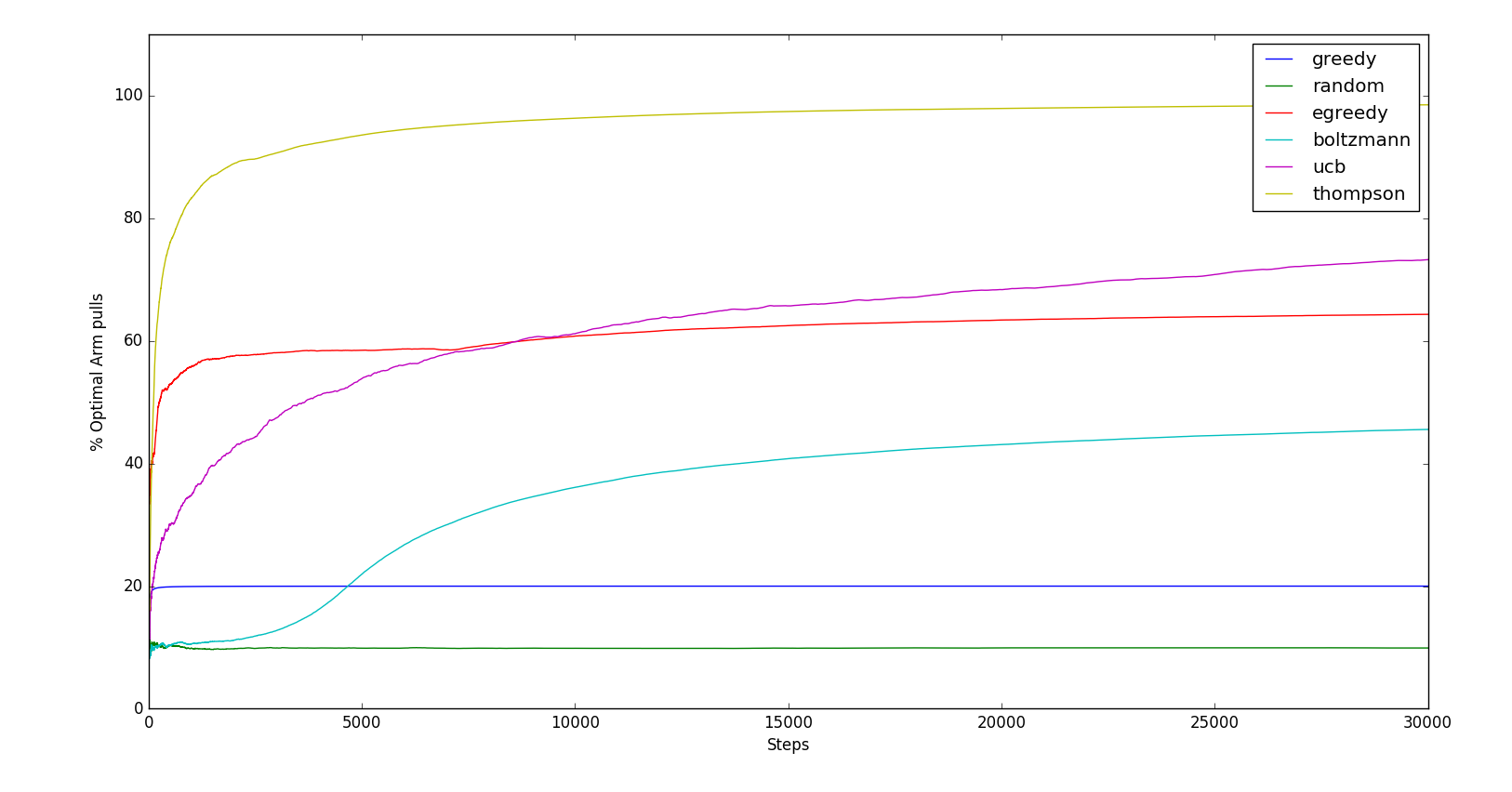
Since we have 10-arms, the Random strategy pulls the optimal arm in only 10% of pulls. Greedy strategy locks onto the optimal arm in only 20% of pulls. The \(\epsilon\)-Greedy strategy quickly finds the optimal arm but only pulls it 60% of the time. UCB is slow to find the optimal arm but then eventually overtakes the \(\epsilon\)-Greedy strategy. Thompson sampling is by far the best strategy, pulling the optimal arm almost 100% of the times. The code for generating this graph and for playing around with Multi armed bandits can be found in this gist.
References: