A Derivation of Backpropagation in Matrix Form
Backpropagation is an algorithm used to train neural networks, used along with an optimization routine such as gradient descent. Gradient descent requires access to the gradient of the loss function with respect to all the weights in the network to perform a weight update, in order to minimize the loss function. Backpropagation computes these gradients in a systematic way. Backpropagation along with Gradient descent is arguably the single most important algorithm for training Deep Neural Networks and could be said to be the driving force behind the recent emergence of Deep Learning.
Any layer of a neural network can be considered as an Affine Transformation followed by application of a non linear function. A vector is received as input and is multiplied with a matrix to produce an output , to which a bias vector may be added before passing the result through an activation function such as sigmoid.
\[Input = x \quad Output = f(Wx+b)\]Consider a neural network with two hidden layer like this one. It has no bias units. We derive forward and backward pass equations in their matrix form.
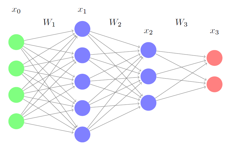
The forward propagation equations are as follows:
\[\mbox{Input} = x_0\\ \mbox{Hidden Layer1 output} = x_1 = f_1(W_1x_0)\\ \mbox{Hidden Layer2 output} = x_2 = f_2(W_2x_1)\\ \mbox{Output} = x_3 = f_3(W_3x_2)\]To train this neural network, you could either use Batch gradient descent or Stochastic gradient descent. Stochastic gradient descent uses a single instance of data to perform weight updates, whereas the Batch gradient descent uses a a complete batch of data.
For simplicity lets assume this is a multiple regression problem.
Stochastic update loss function: \(E=\frac{1}{2}\|z-t\|_2^2\)
Batch update loss function: \(E=\frac{1}{2}\sum_{i\in Batch}\|z_i-t_i\|_2^2\)
Here \(t\) is the ground truth for that instance.
We will only consider the stochastic update loss function. All the results hold for the batch version as well.
Let us look at the loss function from a different perspective. Given an input \(x_0\), output \(x_3\) is determined by \(W_1,W_2\) and \(W_3\). So the only tuneable parameters in \(E\) are \(W_1,W_2\) and \(W_3\). To reduce the value of the error function, we have to change these weights in the negative direction of the gradient of the loss function with respect to these weights.
\[w = w - \alpha_w \frac{\partial E}{\partial w} \quad \quad \mbox{for all the weights } w\]Here \(\alpha_w\) is a scalar for this particular weight, called the learning rate. Its value is decided by the optimization technique used. I highly recommend reading An overview of gradient descent optimization algorithms for more information about various gradient decent techniques and learning rates.
Backpropagation equations can be derived by repeatedly applying the chain rule. First we derive these for the weights in \(W_3\):
\[\begin{align*} \frac{\partial E}{\partial W_3} &= (x_3-t)\frac{\partial x_3}{\partial W_3} \\ &=[(x_3-t)\circ f_3'(W_3x_2)]\frac{\partial W_3x_2}{\partial W_3}\\ &=[(x_3-t)\circ f_3'(W_3x_2)]x_2^T\\ \mbox{Let }\delta_3 &= (x_3-t)\circ f_3'(W_3x_2)\\ \frac{\partial E}{\partial W_3} &=\delta_3x_2^T \end{align*}\]Here \(\circ\) is the Hadamard product. Lets sanity check this by looking at the dimensionalities. \(\frac{\partial E}{\partial W_3}\) must have the same dimensions as \(W_3\). \(W_3\)’s dimensions are \(2 \times 3\). Dimensions of \((x_3-t)\) is \(2 \times 1\) and \(f_3'(W_3x_2)\) is also \(2 \times 1\), so \(\delta_3\) is also \(2 \times 1\). \(x_2\) is \(3 \times 1\), so dimensions of \(\delta_3x_2^T\) is \(2\times3\), which is the same as \(W_3\).
Now for the weights in \(W_2\):
\[\begin{align*} \frac{\partial E}{\partial W_2} &= (x_3-t)\frac{\partial x_3}{\partial W_2} \\ &=[(x_3-t)\circ f_3'(W_3x_2)]\frac{\partial (W_3x_2)}{\partial W_2}\\ &=\delta_3\frac{\partial (W_3x_2)}{\partial W_2}\\ &=W_3^T\delta_3\frac{\partial x_2}{\partial W_2}\\ &=[W_3^T\delta_3 \circ f_2'(W_2x_1)]\frac{\partial W_2x_1}{\partial W_2}\\ &=\delta_2x_1^T\\ \end{align*}\]Lets sanity check this too. \(W_2\)’s dimensions are \(3 \times 5\). \(\delta_3\) is \(2 \times 1\) and \(W_3\) is \(2 \times 3\), so \(W_3^T\delta_3\) is \(3 \times 1\). \(f_2'(W_2x_1)\) is \(3 \times 1\), so \(\delta_2\) is also \(3 \times 1\). \(x_1\) is \(5 \times 1\), so \(\delta_2x_1^T\) is \(3 \times 5\). So this checks out to be the same.
Similarly for \(W_1\):
\[\begin{align*} \frac{\partial E}{\partial W_1} &=[W_2^T\delta_2 \circ f_1'(W_1x_0)]x_0^T\\ &=\delta_1x_0^T \end{align*}\]We can observe a recursive pattern emerging in the backpropagation equations. The Forward and Backward passes can be summarized as below:
The neural network has \(L\) layers. \(x_0\) is the input vector, \(x_L\) is the output vector and \(t\) is the truth vector. The weight matrices are \(W_1,W_2,..,W_L\) and activation functions are \(f_1,f_2,..,f_L\).
Forward Pass:
\[\begin{align*} x_i &= f_i(W_ix_{i-1})\\ E&=\frac{1}{2}\|x_L-t\|_2^2 \end{align*}\]Backward Pass:
\[\begin{align*} \delta_L&= (x_L-t)\circ f_L'(W_Lx_{L-1})\\ \delta_i &= W_{i+1}^T\delta_{i+1}\circ f_i'(W_ix_{i-1})\\ \end{align*}\]Weight Update:
\[\begin{align*} \frac{\partial E}{\partial W_i}&=\delta_ix_{i-1}^T\\ W_i&=W_i - \alpha_{W_i}\circ \frac{\partial E}{\partial W_i} \end{align*}\]Equations for Backpropagation, represented using matrices have two advantages.
One could easily convert these equations to code using either Numpy in Python or Matlab. It is much closer to the way neural networks are implemented in libraries. Using matrix operations speeds up the implementation as one could use high performance matrix primitives from BLAS. GPUs are also suitable for matrix computations as they are suitable for parallelization.
The matrix version of Backpropagation is intuitive to derive and easy to remember as it avoids the confusing and cluttering derivations involving summations and multiple subscripts.
I show a different derivation of Backpropagation in my new post, Yet Another Derivation of Backpropagation in Matrix Form (this time using Adjoints).