Bayesian Inference and the bliss of Conjugate Priors
This blog post is about Bayesian Inference. It finds extensive use in several Machine learning algorithms and applications. Bayesian Inference, along with Frequentist Inference are the two main approaches to Statistical Inference.
For Bayesian Inference, we maintains a probability distribution over possible hypotheses and use Bayes’ Theorem to update the probability for a hypothesis as more data becomes available. The Bayes’ Theorem applicable for inference can be stated as follows:
Let \(\mathbb{H}\) be the set of all hypotheses. \(H\) is a random variable which represents the hypothesis \(h\in \mathbb{H}\) being considered. Random variable \(D\) represents the data seen \(d\).
\[\Pr(H=h\mid D=d) = \frac{\Pr(D=d\mid H=h)\Pr(H=h)}{\Pr(D=d)}\]\(\Pr(H=h)\) is the Prior probability. It expresses the belief about a hypothesis before seeing any data.
\(\Pr(D=d\mid H=h)\) is the Likelihood. It expresses the probability of data \(d\) being generated by hypothesis \(h\).
\(\Pr(D=d)\) is the Marginal Likelihood. It expresses the probability of data \(d\) being generated by any hypothesis from \(\mathbb{H}\). It can also be written as a summation of the product of likelihoods and priors.
\[\Pr(D=d) = \sum_{h \in \mathbb{H}} \Pr(D=d\mid H=h)\Pr(H=h)\]\({\Pr(H=h\mid D=d)}\) is the Posterior probability. It expresses the belief about a hypothesis after the data has been seen.
Now lets apply Bayesian inference to a simple problem of coin tossing. We have a coin which may be tampered. We have to flip the coin \(K\) times and estimate its bias - \(p\)(probability of getting a heads).
Let \(x_i\) be the random variable which is \(1\) when a heads comes up on the \(i\)‘th flip or \(0\) otherwise.
Lets try a Frequentist approach first
After \(K\) flips, \(\sum_{i=1}^Kx_i\) is the number of heads seen. The estimated bias will be:
\[\hat{p}=\frac{\sum_{i=1}^Kx_i}{K}\]After this, we could employ a concentration inequality such as Hoeffdings’s and estimate how close \(\hat{p}\) is to the true bias \(p\).
\[\Pr(\mid \hat{p}-p\mid \ge \epsilon) \le 2\exp(-2K\epsilon^2)\]I have written more about Hoeffding’s inequality in my previous post.
Now the Bayesian approach
Let \(P\) be the continuous random variable for the bias \(p\), whose range is \([0,1]\). Before flipping the coin, we do not know anything about \(p\), except that it could take any value between \(1\) and \(0\). In this case we can assume a Uniform Prior over its range. The probability density function in this case is:
\[f(p) = \begin{cases} 1, & \mbox{if }p \in [0,1] \\ 0, & \mbox{otherwise} \end{cases}\]After the first coin flip, we know the value of \(x_1\). Now we apply Bayes’s Theorem to find the posterior probability density.
\[f(p\mid x_1) = \frac{\Pr(x_1\mid P=p)f(p)}{\Pr(x_1)}\]Since \(x_1\) is a Bernoulli random variable, \(\Pr(x_1\mid P=p) = p^{x_1}(1-p)^{1-x_1}\). Since we assumed uniform priors, \(f(p)=1\). The denominator, \(\Pr(x_1)\) can be expressed as an integration:
\[\begin{align} \Pr(x_1) &= \int_{0}^{1} \Pr(x_1\mid P=p)f(p) dp\\ &=\int_{0}^{1}p^{x_1}(1-p)^{1-x_1}dp \end{align}\]The Beta function is defined as: \(B (x,y)=\int _{0}^{1}t^{x-1}(1-t)^{y-1}d t\).
The Beta distribution is defined as: \(Beta(p;a,b)=\frac{p^{a-1}(1-p)^{b-1}}{B(a,b)}\). So,
\[\Pr(x_1) = B(x_1+1,2-x_1)\]This implies,
\[f(p\mid x_1)=\frac{p^{x_1}(1-p)^{1-x_1}}{B(x_1+1,2-x_1)}=Beta(p;x_1+1, 2-x_1)\]\(f(p\mid x_1)\) is the density of the Beta Distribution with parameters \(x_1+1\) and \(2-x_1\).
After the second flip, we know \(x_2\). Now we can use \(f(p\mid x_1)\) as the prior density and find the new posterior density using Bayes’ Theorem.
\[\begin{align} f(p\mid x_1,x_2) &= \frac{\Pr(x_2\mid P=p,x_1)f(p\mid x_1)}{\int_{0}^{1} \Pr(x_2\mid P=p,x_1)f(p\mid x_1) dp}\\ &=\frac{p^{x_2}(1-p)^{1-x_2}\frac{p^{x_1}(1-p)^{1-x_1}}{B(x_1+1,2-x_1)}}{\int_{0}^{1}p^{x_2}(1-p)^{1-x_2}\frac{p^{x_1}(1-p)^{1-x_1}}{B(x_1+1,2-x_1)}dp}\\ &=\frac{p^{x_1+x_2}(1-p)^{2-x_1-x_2}}{\int_{0}^{1}p^{x_1+x_2}(1-p)^{2-x_1-x_2}dp}\\ &=\frac{p^{x_1+x_2}(1-p)^{2-x_1-x_2}}{B(x_1+x_2+1,3-x_1-x_2)}\\ &=Beta(p;x_1+x_2+1,3-x_1-x_2) \end{align}\]Now we use \(f(p\mid x_1,x_2)\) as the prior for finding the posterior after the third flip. By applying Bayes’ Theorem to all the subsequent coin flips:
\[\begin{align} f(p\mid x_1,x_2,..,x_K) &= Beta(p;1+\sum_{i=1}^Kx_i,K+1 -\sum_{i=1}^Kx_i )\\ f(p\mid x_1,x_2,..,x_K) &= Beta(p;1+\mbox{Number of Heads },1 + \mbox{Number of Tails }) \end{align}\]The mean of the Beta distribution \(Beta(x;a,b)\) is \(\frac{a}{a+b}\). Since \(p\) is distributed according to a Beta distribution, its mean value is:
\[E[p] = \frac{1+\sum_{i=1}^Kx_i}{K+2}\]Note that this is different from the empirical mean in the frequentist case, but both of them approach the true bias in the limit (infinite trials).
Another interesting thing to note: The posterior distribution \(f(p\mid x_1,x_2,..,x_K)\) holds even when we have seen no samples at all. It is simply the uniform distribution.
\[f(p)=Beta(p;1,1)=U(p;0,1)\]Every time we apply Bayes’ Theorem, the Prior and Posterior distributions are Betas and the Likelihood is Bernoulli. Whenever the prior and posterior belong to the same family of distributions, we call the prior and posterior as Conjugate Distributions, and the prior is called a Conjugate Prior for the likelihood function. This is the Conjugacy property of probability distributions. Having a conjugate prior for a likelihood greatly simplifies Bayesian inference as the posterior is obtained by updating the parameters of the prior.
\[\begin{align} f(p)&=Beta(p;1,1)\\ f(p\mid x_1)&=Beta(p;x_1+1, 2-x_1)\\ \vdots\\ f(p\mid x_1,x_2,..,x_K) &= Beta(p;1+\sum_{i=1}^Kx_i,K+1 -\sum_{i=1}^Kx_i ) \end{align}\]In my previous post: Die rolls and Concentration Inequalities, I took a frequentist approach by using the empirical means to approximate the true distribution and then derived a PAC bound for it. We could also take a Bayesian approach. In this case, the Likelihood is the Categorical Distribution and the Prior is the Dirichlet Distribution, which is also the categorical distribution’s conjugate prior.
Restating the problem again: You have an \(n\)-sided die, but you do not know if it is a fair one or not. You have to roll the die \(K\) times and estimate its probability distribution.
Assume the faces are numbered \(1,2,..n\). Let the true probability that face \(i\) comes up when the die is rolled be \(p_i\). Let \(x_{i,t}\) be the indicator variable defined as follows:
\[x_{i,t}= \begin{cases} 1, & \mbox{if } \mbox{face } i \mbox{ comes up on roll } t \\ 0, & \mbox{otherwise} \end{cases}\]Let \(x_t=(x_{1,t},x_{2,t},...x_{n,t})\) and \(\mathbb{I}=(1,1,...1)\). The probability vector \(p=(p_1,p_2,..p_n)\) of the die is distributed according to the Dirichlet distribution as follows:
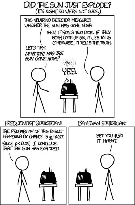
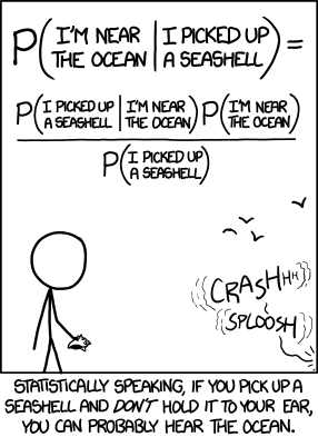
\[\begin{align} f(p)&=Dirichlet(p;\mathbb{I})\\ f(p\mid x_1)&=Dirichlet(p;\mathbb{I}+x_1)\\ \vdots\\ f(p\mid x_1,x_2,..,x_K) &= Dirichlet(p;\mathbb{I}+\sum_{i=1}^Kx_i) \end{align}\]Some related humor from xkcd: